Differentiable Lap Time Simulation with Optimal Control
This page briefly overviews the development of a Lap Time Simulation (LTS) tool using optimisation techniques paired with automatically differentiable dynamics to determine the true limit of race car performance.
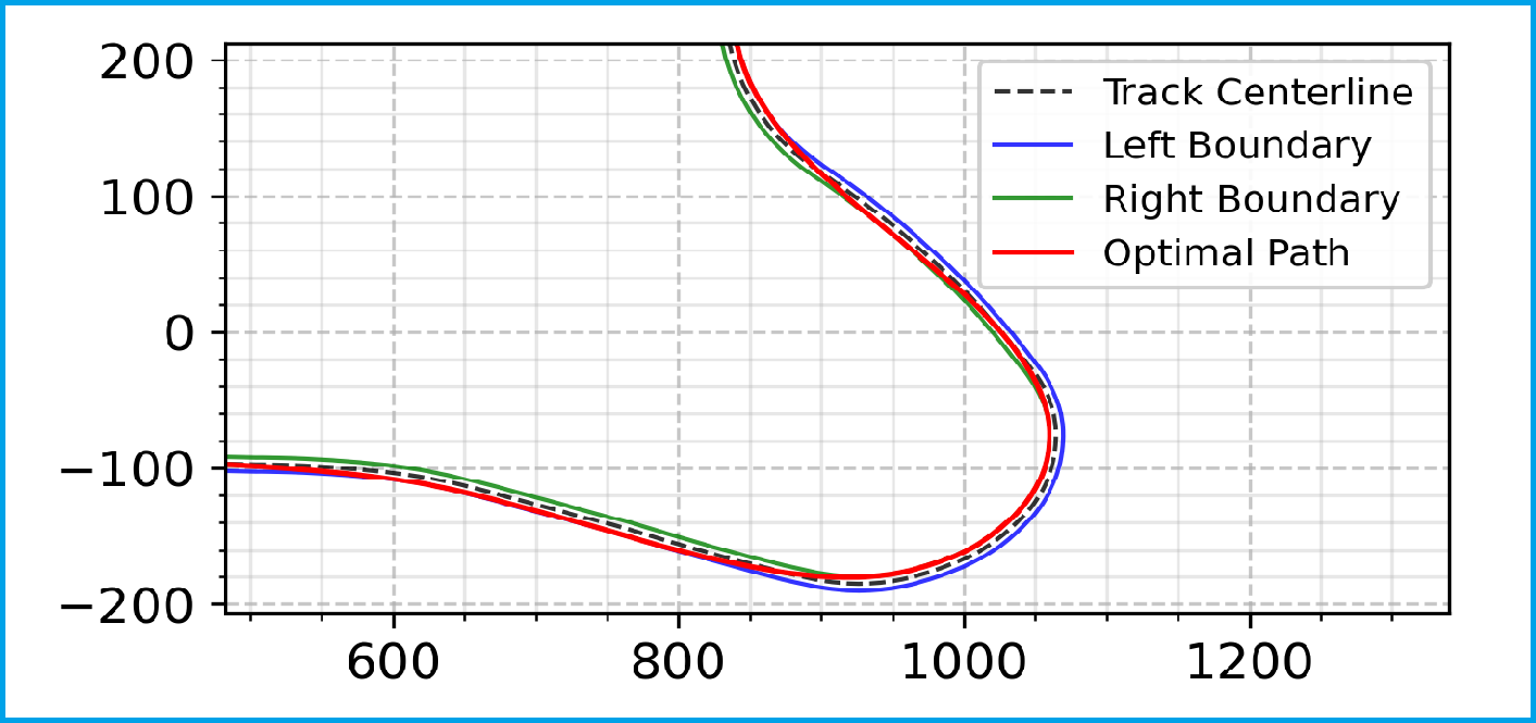
Computed optimal Greenpower racing line at Goodwood's 'Lavant' corner.
When improving Greenpower cars certain directions are obvious, e.g. reduce drag and reduce mass (without compromising safety). However, there are more nuanced engineering decisions that need to be made, such as: what is the optimal way to deploy your limited battery energy around a lap, considering hills, headwinds and corners?
To answer these questions, you either need to do extensive and expensive real-life testing, or detailed physics models representing the cars behaviour must be simulated virtually. In racing this is known as Lap Time Simulation (LTS).
Classical LTS involves integrating the differential equations governing your system forward in time, but these require ‘loop-closure’ methods to provide the control inputs driving your system at each integration time step (throttle/brakes/gears/steering). You can either close the loop with a real driver, like F1 Driver in Loop (DiL) simulators, or you can write some code to try and represent a driver. However, both methods come with a caveat: how do you know that your loop closure method is optimal?
When simulating variables like aerodynamic balance on an F1 car, does the simulated improvement in lap time come from the car being able to extract more grip, or does the specific driver or control code just prefer that setup? If they were to change their driving style could the opposite change in lap time occur? Solving the issue of ‘optimality’ is the current gold standard in LTS – optimal control methods, used extensively in F1.
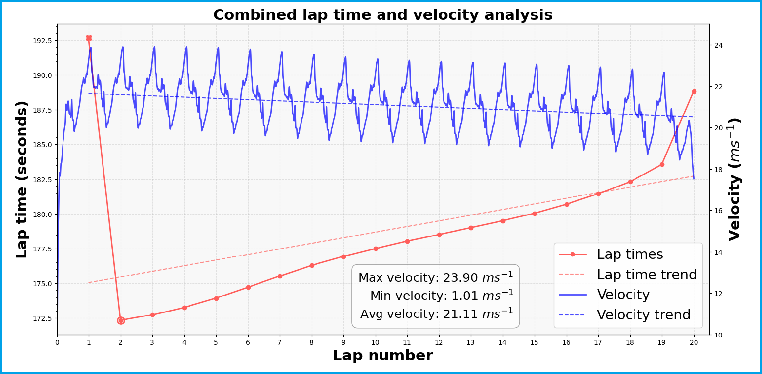
Computed optimal velocity profile (and lap times) over a Greenpower race at Goodwood. The reducing average velocity due to battery voltage degredation is obvious.
As part of my fourth-year dissertation, I wrote an optimal control LTS for Greenpower cars predominantly with Python, making use of CasADi (a framework for automatic differentiation) and opensource large-scale nonlinear optimisation solvers like IPOPT and BONMIN.
Optimal control methods for dynamic simulation involve a shift in perspective on how to simulate. Instead of integrating forward in time the track is discretised into sequential points space, with the car having a full state description at each of these collocation points. This leads to a large collection of state variables. We know that in between each pair of points on the track (a segment) the physics governing the states must be adhered to. Simplified, if we were to look at the state of velocity, we know that between the two points F = ma must be ‘true’ as this is the physics governing the evolution of velocity. We can set that as an equality constraint relating the velocity states at each collocation point. Now we have many state variables and many equality constraints enforcing the correct physical behaviour between these variables.
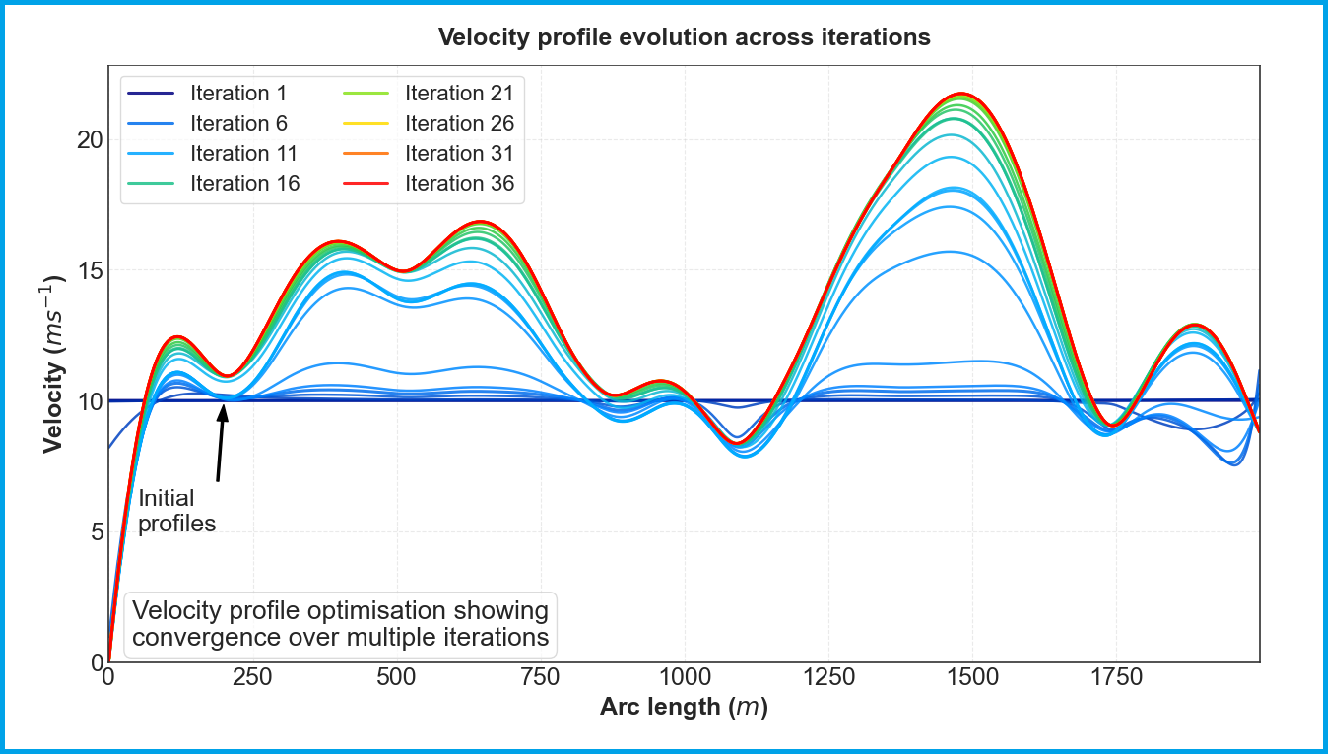
Optimisation solver progression for the state of velocity over the first racing lap starting from a constant 10 m/s initialisation.
This is just a very large optimisation problem, where we are looking to find the minimum lap time by selecting the optimum state variables at each collocation point around the track, making sure to satisfy the physics constraints.
Crucially we can also set the driver’s inputs as control variables in this optimisation problem. If we are certain our optimisation process has found a global solution, then we can be confident that any change in lap time found when making nuanced decisions is real and not a result of how much coffee the Driver in Loop has had.
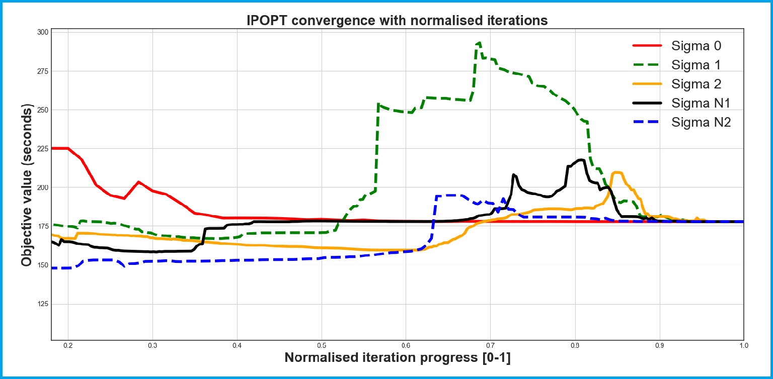
Optimisation solver progression for the lap time (objective function) starting from varying initial conditions. The different colours represent different sized pertubations to the initial conditions, but all converge to the same optimum, providing a level of confidence that this is a robust minimum.
These optimisation problems can be very large, non-linear and non-convex, which means finding global optimums is hard, and even harder to be confident in (as much as one can with only necessary conditions). The specific approach taken in our LTS is a direct collocation approach with trapezoidal quadrature. We write the dynamics such that automatic differentiation can be used to compute gradient and hessian information for solvers, as this is much faster and more reliable than numerical gradient information. This is towards the simpler end of optimal control methods but works well for Greenpower cars where the states change smoothly, not featuring stiff dynamics like grip limited tyres.